Although this page is often accessed as a stand-alone piece, it is part of a work on the history of the British and Irish cement industries, and where statements are made about the historical development of techniques, these usually refer only to developments in Britain.
by chemical analysis, most accurately by x-ray fluorescence spectrometry.
Although the former is most informative about structures that will control the properties of the clinker, it is to no avail if a high-accuracy chemical analysis is not also available. The latter is often lacking.
Microscopy, although of limited application on its own, and prone to error due to the subjective judgment of the microscopist, is of value at least for illustration of the structure of clinker, and vividly-coloured microscopy images, of more decorative value than utility, adorn every cement laboratory, and are proudly displayed for the admiration of visitors. The equipment used is relatively inexpensive, but the labour cost is high, and if sufficiently frequent examinations are performed to be statistically valid, is fantastically expensive.
With the employment of electron microscopy, the situation is quite different. By pointing the electron beam at individual crystals within the microscope image, an electron probe microanalysis can be obtained which, in addition to unambiguously identifying the mineral in question, can also give information on minor elements present. This process can be automated to obtain objective data on the sample. As yet, it remains a "research-only" technique.
X-ray diffraction equipment is becoming more common on cement plants, and can be relatively cheap in capital cost - less than £60,000 - but is effective only in combination with sophisticated - and expensive - software to perform automated Rietveld analysis.
X-ray fluorescence spectrometry is the standard method of chemical analysis of cement systems. Although relatively cheap instruments can be obtained, instruments of the necessary accuracy are expensive - over £200,000 - and sample preparation equipment of the required quality can cost as much again.
The visible-light microscopy techniques used in the cement industry had their origins in the work of various French researchers in the late eighteenth century, who started looking at powdered rock under the microscope in order to identify and quantify its mineral constituents. Nicol, in 1831, described a method of obtaining transparent, ultra-thin sections of rock for examination with transmitted light. The technique remained a mere curiosity until Henry Clifton Sorby of Sheffield in 1858 published systematic work on thin sections of a wide variety of rocks and established the science of petrography. In service to the local steel industry, he went on to look at metals, using polished and etched sections viewed in reflected light, publishing this in 1864. By this stage, most of the subsequently used techniques were laid down.
The application to cement technology began when Henri Louis Le Châtelier in France in the 1880s started making thin sections of clinker. In these he described the four main phases, and established their chemical identity. Törnebohm in 1897 gave the phases their mineral names. In the early twentieth century, with the ascendency of the American industry, most of the significant developments took place in the USA. Campbell gives a good account of this. As early as 1905, cement reactivity was being correlated with phase crystal size and form. Polished sections viewed in reflected light were first attempted in 1908, but were not used until 1934, when Tavasci described a wide range of techniques still in general use today.
The polished section, etched with a variety of reagents to accentuate different features, and viewed in reflected polarized light, is the mainstay of microscopy work today. Without going into detail (all of which can be obtained from Campbell), a typical sample preparation technique consists of the following stages:
place crushed or whole clinker nodules in a glass or plastic vial around 25 mm in diameter
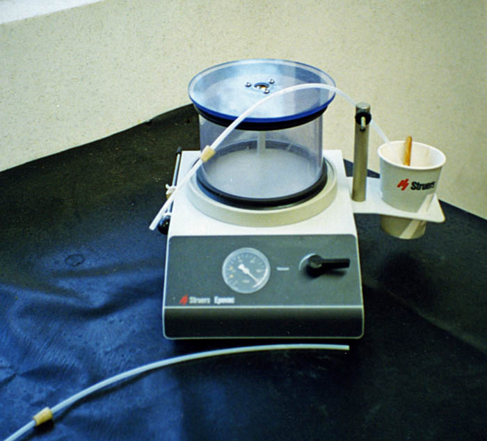
place the vial under vacuum and add a liquid resin, usually epoxy, and repeatedly release and apply vacuum so that the resin penetrates most of the pores in the clinker
allow the resin to harden at 40-60°C
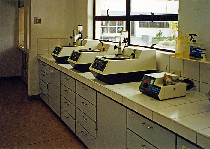
remove the vial and cut through the block of resin with a diamond saw, sectioning the clinker particles
grind the exposed surface flat on a lapping wheel using successively finer abrasives (starting with 50 μm carborundum and finishing with 0.3 μm diamond, corundum or rouge), using a non-aqueous liquid lubricant, typically 1,2-propanediol
wash the surface clean with a volatile non-aqueous solvent and allow to dry
apply and remove etchants, wash and dry
Vacuum impregnator used to embed the clinker sample in resin. Resin mixed in the cup can be injected into the samples while under vacuum.
Equipment for obtaining a flat cross-section of the sample. Right: diamond saw. Left: lapping wheels with three grades of abrasive.
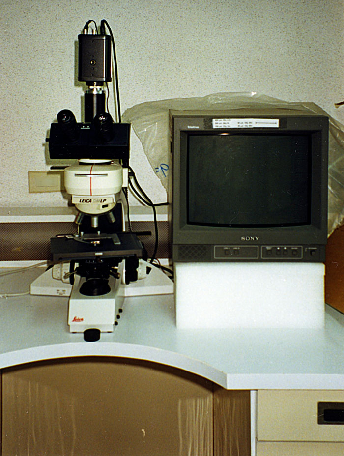
Microscope for examining samples in reflection or transmission mode, and equipped with polarized light source.
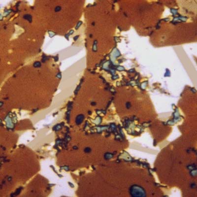
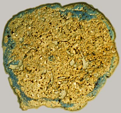
The specimen is viewed under the microscope, with typical magnifications 100-400. Many of the minerals present can be identified visually. The micrograph image, as well as confirming – as it must – the overall chemistry of the clinker, yields information on the homogeneity of the chemical system, and gives clues as to the thermal regime to which it has been subjected. For example, belite crystals well distributed among the preponderance of alite shows good rawmix homogeneity. Over-large alite crystals indicate too-hot burning. Large, well-formed crystals of aluminate and ferrite indicate too-slow cooling.
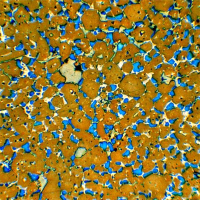
Showing belite (blue) well distributed among alite (orange). Aluminate and ferrite are white/grey, voids are buff grey. View 0.2 mm across
Showing slowly cooled clinker. Well formed crystals of ferrite (white) and alkali-modified aluminate (grey) occupy the space between the silicates. The alite is decomposing along its edges to belite. View 0.08 mm across
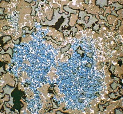
Showing dense concentration of pure belite caused by a large particle of unground sand in the rawmix. View 0.2 mm across
Showing concentration of belite interspersed with aluminate caused by a large shale particle in the rawmix. View 0.2 mm across
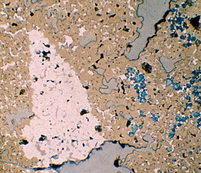
Showing a mass of free lime (pinkish) resulting from a large (0.15 mm) chip of limestone in the rawmix. View 0.2 mm across
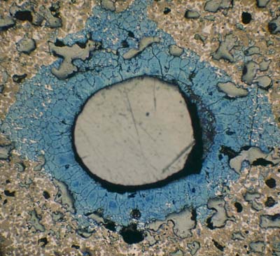
Showing the effect of late coal ash deposition on an entire clinker nodule, causing a concentration of belite on the outside. View 10 mm across
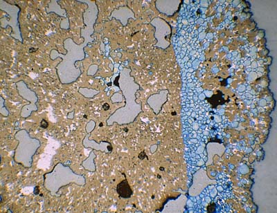
Showing the same effect near the nodule edge in close-up. Several other "layering" effects and patches of free lime can be seen. View 0.2 mm across
The idea that crystals could act as diffraction gratings for x-rays was first put forward by von Laue early in 1912. The idea attracted numerous stellar names in the world of physics, and before the end of 1912, the Braggs had used it to establish the structure of sodium chloride. By 1914, Debye had demonstrated powder diffraction. Gradual advance in the intensity of x-ray sources and improvements in detectors by 1930 allowed Brownmiller and Bogue to perform powder diffraction analyses of Portland cement clinker.
The technique involves grinding a sample down to the 1-5 μm size range, carefully pressing it into a “compact” with a flat faced surface, and directing a collimated beam of monochromatic x-rays onto the surface. At certain discrete angles of incidence, sharp “reflections” are produced, each characteristic of the distance between crystal planes of one of the minerals present. The position of these “diffraction lines” is related to the inter-plane distance by the Bragg Law:
sinθ = nλ/2d
θ is the angle of incidence to the flat sample surface (zero = perpendicular)
λ is the X-ray wavelength
d is the distance between crystal planes
n is the “reflection order” – a positive integer
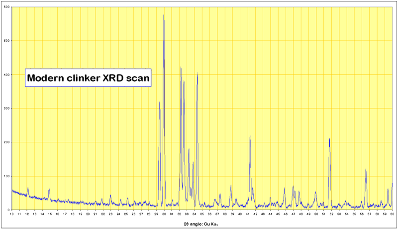
Not surprisingly, most of the prominent lines are those of alite and belite.
So if Cu Kα x-rays are used (as is usually the case), having a wavelength of 0.15418 nm, and a line is found at an incident angle of 9.65°, then provided that the reflection order is 1 (which it usually is for strong lines) the “d-spacing” is 0.460 nm. Since every crystal has multiple planes in its structure, and many types of crystal may be present, the resulting diffractogram consists of a forest of peaks.
Simple qualitative analysis can be done by simply “eyeballing” the diffractogram and recognising patterns. Early attempts at using the data quantitatively were based on measurement of a single, strong peak for each mineral present, but this was always subject to errors due to line overlap, absorption and the effects of solid solution in the minerals, so that precision was always mediocre at best. Modern practice uses highly computer-intensive curve-fitting on the entire diffractogram, making allowance for variable background, changes in line-shape, and adjustment of crystal cell parameters. This yields precision superior to microscopic point-counting, although the process as yet is still too slow for quality control work, and requires supervisory expertise. Modern technical developments also include the use of synchrotrons instead of conventional x-ray tubes, allowing much better signal/noise ratio and better resolution, and the advent of solid state array detectors that allow the scan of incident angles to be acquired much faster.
Chemical Analysis
The measurement of chemical composition is the oldest and still the most important means of characterising cement materials and controlling the manufacturing process. However, analysis to a high degree of precision and accuracy is a relatively modern practice, and even today is often lacking. Jackson gives an excellent history of the development of “standard” methods, and shows how, up to the present, details of analysis which have a very significant effect upon the result continue to be argued about. To understand this, it is necessary to recognise three distinct conflicting approaches that have always been a feature of the problem:
Research-grade analysis, which aims to establish the accurate elemental composition of a material: the British cement industry has rarely, if at all, availed itself of this.
Analysis for demonstrating compliance with a standard specification, which generally involves producing data in a specified manner, agreed by consensus within the industry, although not necessarily informed by any science.
Analysis for control purposes, the aim of which is solely to make a cement consistently with the desired physical properties, which occupies a spectrum of techniques which may vary from the highest technology down to rule-of-thumb techniques devoid of any chemistry.
As Jackson shows, although the first British Standard for Portland cement (BS12) in 1904 required various chemical parameters to be measured, no guidance was given on how this was to be done, and apart from a method for measuring acid insoluble material content (1947), no procedures were specified until as late as 1970 – by which time most of the techniques specified had been superseded in practice. However, all the early texts on cement manufacture include lengthy sections on how to analyse cements and raw materials. These were almost invariably the personal methods of the authors, who were to a greater or lesser degree involved with the practicalities of control, so that the methods often involved short-cuts and compromises that have a major effect upon the results. For this reason, in making historical comparisons on trends in cement chemistry, great caution and scepticism is necessary. Straightforward compositional parameters such as CaO, SiO2 and SO3 content have significant biases depending on the methods used, while other important parameters can very easily be out by a factor of two or more. A systematic approach to the history involves “calibrating” the data of prolific analysts such as Butler and Spackman, making allowance for the likely biases and using knowledge of more modern analyses of the materials they looked at.
The early analyses were all based upon classical “wet” methods involving dissolution of the material, then estimating components gravimetrically – i.e. by precipitating and weighing them – or volumetrically by titration with a reagent that reacts with the element in question. Without going into excessive detail, the most important parts of the analysis scheme consisted of:
Dissolving the sample in acid (properly made clinker dissolves in hydrochloric acid very easily and completely).
Weigh what little fails to dissolve as "insoluble residue".
Reduce the pH to precipitate silica: ignite and weigh it.
Neutralize with ammonia, precipitating "R2O3" - consisting of most of the Al2O3, Fe2O3, TiO2, P2O5 and Mn2O3. This is ignited and weighed.
Add ammonium oxalate to precipitate calcium oxalate: ignite it to CaO and weigh.
Concentrate the remaining solution and add ammonium phosphate to precipitate MgNH4PO4: ignite it to Mg2P2O7 and weigh.
Redissolve the "R2O3" in acid and separately determine Fe2O3 by selective precipitation or by a redox reaction.
The last stage was often missed out in early analyses. SO3 was measured on a fresh sample by precipitation as BaSO4. This was a typical cement plant analysis: from early times, more scientific investigations performed additional analysis for Na, P, Cl, K, Ti, Mn, Zn, Sr, Ba, etc. No even moderately accurate method of analysis for Al2O3 existed until the arrival of XRF in the 1960s. Reliable alkali metal analysis remained quite inaccessible until flame photometry was introduced. One glaring omission from early analysis was any estimation of the amount of "free" or "uncombined" CaO in clinker. A method was developed in the USA in 1920s involving non-aqueous dissolution and titration of the free CaO using glycols in an alcohol solvent. A variant finally came into use in Britain after WWII. For many years prior to this it was often claimed that there was no free lime in cement - a claim very wide of the mark. Early manufacturers often "matured" their cement for several months before daring to sell it, to give time for the free lime to hydrate.
Accurate analysis only started to develop as “instrumental” techniques became available – and in particular, various spectrometric techniques that provided absolutely element-specific data. Among these, atomic emission and absorption techniques were used, but overwhelmingly the most important is x-ray fluorescence spectrometry.
Even with highly automated instrumental techniques, accurate analysis of cement is particularly difficult. The analysis problem is subtly different from that of most other process materials. Other major products for which chemistry is important – for example iron or aluminium – usually consist largely of a single element or compound in which the other constituents are only present in minor or trace quantities. At worst, an alloy may be a simple binary mixture. The minor constituents can be measured in the knowledge that the remaining “background” material is constant and well characterised. “Spiking” techniques can be used with confidence to measure traces. Cement, on the other hand, is always a complex mixture in which the analysis of an individual component is subject to interference from many other components, most of which can have a wide range of concentrations. In the production of research-grade, high accuracy analyses, the favoured technique is to split the material into moderately pure components by gravimetric methods, then analyse each of these by instrumental methods, quantifying the contaminants as traces, then re-assemble the analysis of the original material. This approach began to be used in the 1960s, and since then, accurately characterised reference materials have been available for calibrating instrumental analysis systems.